
Coalescent simulation in python, a brief introduction
This blog is an introduction to two python modules, msprime (by Jerome Kelleher) and scikit-allel (by Alistair Miles), both of whom are based in Oxford at the Big Data Institute. They are both really great tools, and if you work with genomic data I would encourage you to take a look at them.
However, the particular point I’d like to make here is that they work really nicely together.
msprime is a coalescent simulator with a python interface, essentially an efficient version of ms, that also writes data in a sensible format, a compressed sequence tree rather than text files that need to be parsed (which are the bane of bioinformaticians).
scikit-allel is a toolkit for working with genomic data. Crucially it abstracts data chunking and compression allowing handling of extremely large datasets on a desktop machine. It has a wealth of functions, and is very fast.
It’s easy to imagine taking several days to construct and debug an ms command, parse the results into something plink can work with, compute summary statistics, then parse that into a format appropriate for a plotting library. What I will show here is that this is possible in a few very readable lines of python.
Writing your own parsing code is prone to bugs, even for experienced coders. It’s almost invariably inefficient, and harder to maintain/reproduce when you have several tools in your chain.
Here comes some code…
We begin as usual by importing some essential libraries. As well as the two that are the subject of this blog, we use numpy to create a format from msprime that allel can understand, pandas for handling tabular data, and the seaborn wrapper to matplotlib for plotting.
import allel
import msprime
import seaborn as sns
import pandas as pd
import numpy as np
%matplotlib inline
assert msprime.__version__ == "0.4.0"
assert allel.__version__ == "1.1.9"Overview
The task I am going to work though is to simulate two populations, with different demographic histories, and see how genome summary statistics differ.
-
We’ll draw 100 samples from a population size of 1000. Both populations have experienced bottlenecks, one very rapid, the other a gradual decline over many generations.
-
Population 1 has experienced a crash starting 40 generations ago, until 20 generations ago, declining at 25% per generation.
-
Poputation 2 has experienced a 0.5% per generation decline for 1000 generations. Both have been stable for 20 generations.
Obviously here we can specify more complex demographic scenarios as needed!
history_p1 = [
    msprime.PopulationParametersChange(time=20, growth_rate=-0.25, population_id=0),
    msprime.PopulationParametersChange(time=40, growth_rate=0, population_id=0)]
history_p2 = [
msprime.PopulationParametersChange(time=20, growth_rate=-0.005, population_id=0),
msprime.PopulationParametersChange(time=1020, growth_rate=0, population_id=0)]pop_config = [msprime.PopulationConfiguration(
sample_size=100, initial_size=1000, growth_rate=0)]msprime also has this neat demography debugger feature so we can check the demographic history is as we intended.
dp = msprime.DemographyDebugger(population_configurations=pop_config,
                                demographic_events=history_p1)

dp.print_history()
============================
Epoch: 0 -- 20.0 generations
============================
start end growth_rate | 0
-------- -------- -------- | --------
0 | 1e+03 1e+03 0 | 0
Events @ generation 20.0
- Population parameter change for 0: growth_rate -> -0.25
===============================
Epoch: 20.0 -- 40.0 generations
===============================
start end growth_rate | 0
-------- -------- -------- | --------
0 | 1e+03 1.48e+05 -0.25 | 0
Events @ generation 40.0
- Population parameter change for 0: growth_rate -> 0
==============================
Epoch: 40.0 -- inf generations
==============================
start end growth_rate | 0
-------- -------- -------- | --------
0 |1.48e+05 1.48e+05 0 | 0
dp = msprime.DemographyDebugger(population_configurations=pop_config,
                                demographic_events=history_p2)

dp.print_history()
============================
Epoch: 0 -- 20.0 generations
============================
start end growth_rate | 0
-------- -------- -------- | --------
0 | 1e+03 1e+03 0 | 0
Events @ generation 20.0
- Population parameter change for 0: growth_rate -> -0.005
=================================
Epoch: 20.0 -- 1020.0 generations
=================================
start end growth_rate | 0
-------- -------- -------- | --------
0 | 1e+03 1.48e+05 -0.005 | 0
Events @ generation 1020.0
- Population parameter change for 0: growth_rate -> 0
================================
Epoch: 1020.0 -- inf generations
================================
start end growth_rate | 0
-------- -------- -------- | --------
0 |1.48e+05 1.48e+05 0 | 0
This function is the key part, and represents the interface between the two tools. I’ve tried to explain what’s happening in the comments
def growth_dem_model(pop_cfg, dem_hist, length=1e7, mu=3.5e-9, rrate=1e-8, seed=42):


    # call to msprime simulate method. This returns a generator of tree sequences.
    # One gotcha I found is that the object returned is different if you use the num_replicates argument
    tree_sequence = msprime.simulate(
        length=length, recombination_rate=rrate,
        mutation_rate=mu, random_seed=seed,
        population_configurations=pop_cfg,
        demographic_events=dem_hist)

    # print the number of mutations in the trees using an internal method
    print("Simulated ", tree_sequence.get_num_mutations(), "mutations")

    # thanks to Jerome for the code here.
    # The best way to do this is to preallocate a numpy array
    # (or even better the allel.HaplotypeArray), and fill it incrementally:
    V = np.zeros((tree_sequence.get_num_mutations(), tree_sequence.get_sample_size()),
                 dtype=np.int8)

    for variant in tree_sequence.variants():
        V[variant.index] = variant.genotypes

    # create a haplotype array in allel from numpy arrays of 0s/1s
    # as the dataset is reasonably small there is no need to use the chunking functionality of allel
    gt = allel.HaplotypeArray(V)

    # scikit-allel expects integer values here rather than infinite sites model of msprime.
    pos = allel.SortedIndex([int(variant.position) for variant in tree_sequence.variants()])

    return gt, pos
We’ll use a contig of 10 Mbp, and summarize the data in 10 kbp windows.
contig_length = 10000000
window_size = 10000%%time
simulations = {"recent_crash": growth_dem_model(pop_config, history_p1, length=contig_length),
"slow_decline": growth_dem_model(pop_config, history_p2, length=contig_length)}Simulated 98234 mutations
Simulated 70472 mutations
CPU times: user 1min 54s, sys: 167 ms, total: 1min 54s
Wall time: 1min 54s
Initialize our data frame: create a multi-index from the combinations of the things we are interested in, and tell it how many rows to expect.
mi = pd.MultiIndex.from_product((simulations.keys(), ("pi", "tajimaD", "wattersonTheta")),
                                names=["scenario", "statistic"])

df = pd.DataFrame(columns=mi, index=range(0, contig_length//window_size))
Using the nice indexing features of pandas it’s simple to write a loop, and save the data in the appropriate index.
allel also returns some other values such as counts, and bin limits, which in this case we are not interested in, so we assign to _.
%time
for key, (haps, pos) in simulations.items():

    pi, _, _, _ = allel.diversity.windowed_diversity(
        pos, haps.count_alleles(), size=window_size, start=0, stop=contig_length)

    df[key, "pi"] = pi

    tjd, _, _ = allel.diversity.windowed_tajima_d(
        pos, haps.count_alleles(), size=window_size, start=0, stop=contig_length)

    df[key, "tajimaD"] = tjd

    watt, _, _, _ = allel.diversity.windowed_watterson_theta(
        pos, haps.count_alleles(), size=window_size, start=0, stop=contig_length)

    df[key, "wattersonTheta"] = watt
CPU times: user 2 µs, sys: 1e+03 ns, total: 3 µs
Wall time: 4.05 µs
from IPython.display import HTML(I haven’t yet figured out how to get multi-index tables to look nice in markdown/html- apologies!)
HTML(df.head().to_html(float_format='%.4f'))| scenario | recent_crash | slow_decline | ||||
|---|---|---|---|---|---|---|
| statistic | pi | tajimaD | wattersonTheta | pi | tajimaD | wattersonTheta |
| 0 | 0.0019 | -0.0356 | 0.0019 | 0.0016 | 1.5078 | 0.0011 |
| 1 | 0.0018 | 0.2704 | 0.0017 | 0.0022 | 1.6559 | 0.0015 |
| 2 | 0.0019 | 0.3512 | 0.0017 | 0.0023 | 1.3548 | 0.0017 |
| 3 | 0.0020 | 0.5189 | 0.0018 | 0.0019 | 1.5628 | 0.0013 |
| 4 | 0.0013 | -0.7073 | 0.0017 | 0.0018 | 1.9320 | 0.0011 |
_ = sns.factorplot(x="scenario", y="value", col="statistic",
                   data=df.melt(), kind="violin", sharey=False)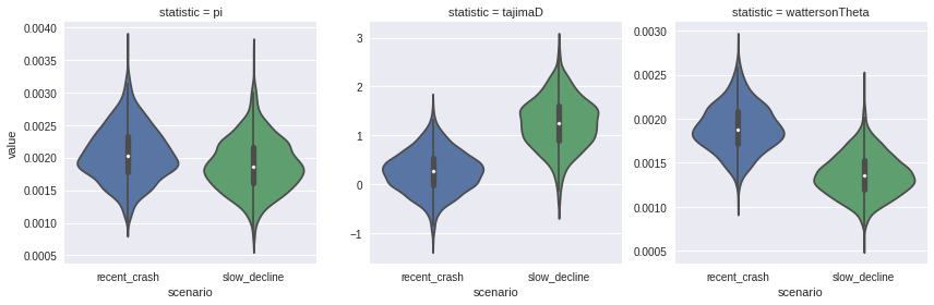
Thanks for reading this far! Hope something was of use.