
Animating population demographic changes
This post animates the genetic signature of a population crash as it unfolds, attempting to shed a little bit more light on when a crash is detectable, and how long it takes to stabilise post-crash.
Although a forward simulation is probably more appropriate here, I chose the extremely fast coalesent simulator msprime. Strictly speaking, the simulations shown here aren’t following a single population crashing, but multiple independent populations at different time periods given a particular demographic history.
msprime is plenty fast enough to handle this type of work, comfortably handling 140 separate coalescent simulations over 10 Mbp in about 90 minutes. Also, the independent observations allow us to visualise the inherent stochasticity present.
The rest of the post details how this was done. But the final animation is shown below:
The left panel shows the demographic history of the population, with the time point currently displayed in the other two panels. In the centre, I show the site frequency spectrum (SFS). This is the distribution of allele frequencies among SNPs present in the population. Under neutrality and a constant population size, we expect rare variants to be observed frequently as they may occur via sporadic mutations- in contrast common variants should be rare, as they take a long time to drift to high frequency. The allele frequency of a polymorphism has a direct relationship to the number of times we may expect to see a polymophism with that allele frequency, a direct consequence of drift. Note that this is independent of the total number of mutations that a population can maintain, the SFS pertains to the relative levels of polymorphisms with different allele frequencies. The SFS therefore encodes information regarding population demographic history; populations that have experienced contraction tend to have a dearth of rare variants, as genetic drift is much more likely to remove these polymorphisms from the population, but insufficient time has passed to generate new mutations.
Here we plot the scaled SFS, where a stable population is expected to show a straight (horizontal) line.
Tajima’s D is a related statistic, and represents the ratio of variation at a per chromosome level to the absolute number of variants in the population.
A negative D suggests an excess of rare variants.
Following the crash we see that even 5000 generations later, the site frequency spectrum hugely disrupted, Tajima’s D is also heavily right skewed.
This is an interesting observation - severe population bottlenecks still leave profound effects on genomes 5000 generations later.
(I explore this a little more thoroughly at the bottom of this page.)
#HTML(html5)from IPython.display import HTMLfrom matplotlib import animation
import matplotlib.pyplot as plt
import seaborn as snsimport os
import numpy as np
import msprime
import math
import allelSimulations begin
If you happened to see my previous post, I wrote about the interface between msprime and scikit-allel, see here. This function is taken directly from that, but with one addition, a cache for previously generated tree sequences. Although msprime is fast, simulating 140 different dempgraphic scenarios takes some time!
def growth_dem_model(pop_cfg, dem_hist, length=1e7, mu=3.5e-9, rrate=1e-8, seed=None,
                     verbose=False, string=None):

    fn = os.path.join("/tmp", string + ".h5")

    if os.path.isfile(fn):
        tree_sequence = msprime.load(fn)
        if verbose:
            print("Loaded tree sequence from file.")
    else:
        # call to msprime simulate method. This returns a generator of tree sequences.
        # One gotcha I found is that the object returned is different if you use the num_replicates argument
        tree_sequence = msprime.simulate(
            length=length, recombination_rate=rrate,
            mutation_rate=mu, random_seed=seed,
            population_configurations=pop_cfg,
            demographic_events=dem_hist)

        tree_sequence.dump(fn)

    # print the number of mutations in the trees using an internal method
    if verbose:
        print("Simulated ", tree_sequence.get_num_mutations(), "mutations")

    # thanks to Jerome for the code here.
    # The best way to do this is to preallocate a numpy array
    # (or even better the allel.HaplotypeArray), and fill it incrementally:
    V = np.zeros((tree_sequence.get_num_mutations(), tree_sequence.get_sample_size()),
                 dtype=np.int8)

    for variant in tree_sequence.variants():
        V[variant.index] = variant.genotypes

    # create a haplotype array in allel from numpy arrays of 0s/1s
    # as the dataset is reasonably small there is no need to use the chunking functionality of allel
    gt = allel.HaplotypeArray(V)

    # scikit-allel expects integer values here rather than infinite sites model of msprime.
    pos = allel.SortedIndex([int(variant.position) for variant in tree_sequence.variants()])

    return gt, pos
Parameters
Here I define recombination rate, mutation rate, and how much DNA I want to simulate.
rrate = 1e-8
mu = 1e-8

window_size = 10000 #bp
contig_size = 10000000 #bp
sample_size = 100 # chromosomes
Specifications
Here I make some intial specifications about the demographic history I wish to simulate… The population is at time t 1000 chromosomes, with a decline of 0.5% per generation for 1000 generations completing at 5000 generations in the past (and therefore starting at 6000 generations in the past).
initial_size = 1000
span = 1000
gen_limit = 7000
growth_rate = -0.005
abs_time = 5000
Now we need to decide at which time points to sample, I chose a gap of 100 generations, reduced to 10 during the population crash. This has the nice effect of having more detail over this time point, as well as slowing down the animation during the interesting bit.
# define the generations to iterate over.
# more time on interesting periods.
generations = np.concatenate(
    [np.arange(0, abs_time, 100),
     np.arange(abs_time, abs_time + span, 10),
     np.arange(abs_time + span, gen_limit, 100)])
generations
array([ 0, 100, 200, 300, 400, 500, 600, 700, 800, 900, 1000,
1100, 1200, 1300, 1400, 1500, 1600, 1700, 1800, 1900, 2000, 2100,
2200, 2300, 2400, 2500, 2600, 2700, 2800, 2900, 3000, 3100, 3200,
3300, 3400, 3500, 3600, 3700, 3800, 3900, 4000, 4100, 4200, 4300,
4400, 4500, 4600, 4700, 4800, 4900, 5000, 5010, 5020, 5030, 5040,
5050, 5060, 5070, 5080, 5090, 5100, 5110, 5120, 5130, 5140, 5150,
5160, 5170, 5180, 5190, 5200, 5210, 5220, 5230, 5240, 5250, 5260,
5270, 5280, 5290, 5300, 5310, 5320, 5330, 5340, 5350, 5360, 5370,
5380, 5390, 5400, 5410, 5420, 5430, 5440, 5450, 5460, 5470, 5480,
5490, 5500, 5510, 5520, 5530, 5540, 5550, 5560, 5570, 5580, 5590,
5600, 5610, 5620, 5630, 5640, 5650, 5660, 5670, 5680, 5690, 5700,
5710, 5720, 5730, 5740, 5750, 5760, 5770, 5780, 5790, 5800, 5810,
5820, 5830, 5840, 5850, 5860, 5870, 5880, 5890, 5900, 5910, 5920,
5930, 5940, 5950, 5960, 5970, 5980, 5990, 6000, 6100, 6200, 6300,
6400, 6500, 6600, 6700, 6800, 6900])
len(generations)160
This is just a quick sum to work out the ancestral size of the population- because we are dealing with the coalescent, we work backwards…
# ancestral size
initial_size * math.exp(-growth_rate * span)
148413.1591025766
size_history = []Here I specify a seed so that the cacheing described above works.
np.random.seed(42)
seeding = np.random.randint(0, 10000, len(generations))
The crash truly happens at 5000 gen - 6000 generations ago. However, we need to adjust the times that are read into msprime, as everything has to be relative. ie at t=1000, then the crash is 4000 generations away, not 5000.
After the simulation we are only interested in the allele counts, so we keep those in a dict.
# we need to recalculate the pop history each loop, as the relative time to crash changes...
ac = {}

for gen, seed in zip(generations, seeding):

    rel_time = abs_time - gen

    # if the crash has not yet occurred. Then fixed pop size
    if (gen > (abs_time + span)):
        history_p = None

    else:
        stability = msprime.PopulationParametersChange(
            time=rel_time + span, growth_rate=0, population_id=0)

        crash = msprime.PopulationParametersChange(
                    time=max(rel_time, 0), growth_rate=growth_rate, population_id=0)

        history_p = [crash, stability]

    # now work out the size of the population at this time.

    # if rel time is positive... then 0.
    if rel_time > 0:
        g_of_crash = 0
    else:
        g_of_crash = min(-rel_time, span)

    size_t = initial_size * math.exp(-growth_rate * g_of_crash)
    size_history.append(size_t)

    pop_config = [msprime.PopulationConfiguration(
        sample_size=sample_size, initial_size=size_t, growth_rate=0)]

    identifier = "sim_s{0}_g{1}".format(seed, gen)

    # now simulate
    haps, pos = growth_dem_model(pop_config, history_p, length=contig_size, mu=mu, rrate=rrate,
                                 seed=int(seed), string=identifier)


    # we are only really interested in allele frequencies...
    ac[gen] = pos, haps.count_alleles()
Using scikit-allel we calculate the scaled site frequency spectrum and Tajima’s D in 10kbp windows. These are stored in dicts to be used later in the animation.
tajima = {}
sfs = {}
for gen, (pos, allele_counts) in ac.items():

    tjd, _, _ = allel.diversity.windowed_tajima_d(
        pos, allele_counts, size=window_size, start=0, stop=contig_size)

    sfs_scaled = allel.sfs_scaled(allele_counts[:, 1])

    tajima[gen] = tjd
    sfs[gen] = sfs_scaled
from functools import reduce# this value used to decide where the y limit is for later plots
max_var = reduce(max, [max(x) for x in sfs.values()])Now animate
n_frames = len(generations)import warnings
warnings.filterwarnings("ignore", category=np.VisibleDeprecationWarning) This is a fairly standard matplotlib animation. It’s not the most efficient, as it redraws the whole axes for the SFS and Tajima’s D plots, but it works well enough here.
These two tutorials were extremely helpful in putting this together:
-
http://jakevdp.github.io/blog/2013/05/12/embedding-matplotlib-animations/
-
https://stackoverflow.com/questions/43552575/how-to-make-a-matplotlib-animated-violinplot
So thanks to the respective authors/answerers.
# First set up the figure, the axis, and the plot element we want to animate
fig, axes = plt.subplots(ncols=3, figsize=(11, 4))

for ax in axes:
    sns.despine(ax=ax, offset=5)

# ax0
ax1, ax2, ax3 = axes
ax1.plot(generations, [val*1e-3 for val in size_history])
ax1.set_ylabel(r"Ne x $10^{3}$")
ax1.set_xlabel("generations")

line1, = ax1.plot([], [])

shapes = [line1]

# initialization function: plot the background of each frame
def init():
    shapes[0].set_data([], [])
    return shapes

# animation function.  This is called sequentially
def animate(i):
    # i is the frame number (to n_gen)

    gen = generations[::-1][i]
    tjd = tajima[gen]
    sfs_scaled = sfs[gen]

    tjd = np.compress(~np.isnan(tjd), tjd)

    # animate line
    shapes[0].set_data((gen, gen), (0, size_history[-1]))

    # animate second
    ax2.clear()

    sns.despine(ax=ax2, offset=5)
    ax2.set_ylim((0, max_var * 1e-3 * 0.75))
    allel.plot_sfs_scaled(sfs_scaled * 1e-3, ax=ax2)
    ax2.set_ylabel(r"scaled site freq. x $10^3$")

    # third
    ax3.clear()
    sns.despine(ax=ax3, offset=5)
    ax3.set_ylabel("density")
    ax3.set_xlabel(r"Tajima's $D$")
    ax3.set_ylim((0, 1.2))
    ax3.set_xlim((-5, 7))

    ax3.vlines([0.0], 0, 1.2, linestyle="--", color="k", lw=1.0)
    sns.distplot(a=tjd, ax=ax3)

    return shapes

# call the animator.  blit=True means only re-draw the parts that have changed.
anim = animation.FuncAnimation(fig, animate, init_func=init,
frames=n_frames, interval=200, blit=True)plt.close()html5 = anim.to_html5_video()
HTML(html5)anim.save("../assets/popcrash.mp4")Is a severe crash detectable 5000 generations later?
To show this I ran two contrasting demographic scenarios. One a population that has been at a constant Ne of 1000 for 5000 generations, but before that experiencing a severe crash from approximately 140,000 over a span of 1000 generations.
The null, alternative model shows a population at a stable Ne of 1000.
The simulation below clearly shows an extremely disrupted site frequency spectrum in the “crash model”.
history_pA = [
    msprime.PopulationParametersChange(time=5000, growth_rate=growth_rate, population_id=0),
    msprime.PopulationParametersChange(time=6000, growth_rate=0, population_id=0)]

history_pB = []


pop_config = [msprime.PopulationConfiguration(
    sample_size=sample_size, initial_size=1000, growth_rate=0)]

seed = 1001
idenA = "5kcrash"
idenB = "nocrash"

# now simulate
hapsA, posA = growth_dem_model(pop_config, history_pA, length=contig_size, mu=mu, rrate=rrate,
                               seed=int(seed), string=idenA)


# now simulate
hapsB, posB = growth_dem_model(pop_config, history_pB, length=contig_size, mu=mu, rrate=rrate,
                               seed=int(seed), string=idenB)

# we are only really interested in allele frequencies...
sfs_a = allel.stats.sfs_scaled(hapsA.count_alleles()[:, 1])
sfs_b = allel.stats.sfs_scaled(hapsB.count_alleles()[:, 1])fig, ax = plt.subplots()
sns.despine(ax=ax, offset=5)
allel.plot_sfs_scaled(sfs_a, ax=ax)
allel.plot_sfs_scaled(sfs_b, ax=ax)
plt.show()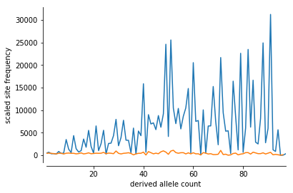
Fin.
Thanks to @alimanfoo for the intial idea, and @jeromekelleher for help with the implementation.